by Stelios Zimeras (University of the Aegean)
In disease spread processes where hidden information dramatically affects the quality of the data, modelling of the spatial patterns is a challenging task. In this situation, models based on spatial structure are important for the investigation of neighbourhood structure between regions where spatial connectivity is defined. We have developed spatial techniques to investigate homogeneity.
Spatial patterns can be explained by modelling the interaction between homogeneous regions or inhomogeneous regions [3]. Spatial models can be defined as specific models where estimation techniques can be applied in regions (in a rectangular or non-rectangular manner) using advanced statistical techniques. These models can be analysed based on Markov random fields where the local neighbouring structure is under investigation. The main concept in spatial analysis is to define the smallest possible areas for the estimation of patterns. This is because regions are composed of a mosaic of textures. Stochastic models and statistical methods have been successfully applied in image analysis. For any statistical analysis that uses such methods, it is vital to choose an appropriate model as the prior and to accurately estimate the prior model parameters.
These local characteristics are defined in terms of the conditional distribution of the random variables at each site, given the values at other sites. This specification is called a Markov random field (MRF). The definition of the MRF came originally from statistical physics, though these processes form a family of Markov processes in which a time index is replaced by a space vector. At this stage, a Markov random field model must be introduced [2]. Markov random fields are defined based on the conditional distributions of the neighbours. As a result, a conditional probability of the pixels, given the neighbours, is introduced with general form given by the Gibbs distribution (e.g. Ising and Potts models) or by auto-models. Models for disease spread are given based on whether the disease succeeds or fails to appear in the region. For this reason, a logistic model could be used with white patches representing success and black representing failure. Due to the 2D definition of the region and the conditionality of the pixel values, these models are defined as auto-models (Figure 1).
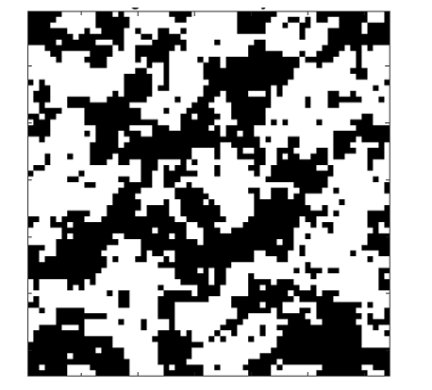
Figure 1: Auto-logistic model of disease spread. The white pixels show where the disease has appeared and black is the background.
A homogeneous auto-logistic model (Ising model), assuming uniform temperature, is shown in Figure 2. Texture analysis focuses on extraction information based on sufficient features to characterise real texture images. By representing a complex real texture via statistical methods or parameters, texture analysis becomes an important tool to explain specific phenomena.

Figure 2: An auto-logistic model of disease of disease spread. The images show realizations from Ising model: 3 iterations, 25 iterations, and 100 iterations from the Ising model.
Uncertainty can present a major problem when analysing incomplete data, especially in spatial modelling at different spatial and temporal scales. Uncertainty analysis, in this context, is the process of assessing uncertainty in modelling or scaling to identify its major sources, quantify their degree and relative importance, examine their effects on model output under different scenarios, and determine prediction accuracy. Inherent in the modelling process is the introduction of statistical errors (especially in spatial modelling where homogeneity of the neighbours is one of the measures to justify differences between regions). Incomplete datasets, spatial differences and statistical modelling all contribute to the complexity of analysing uncertainties in regions.
Although the issues with uncertainty analysis can be considered to be analogous to standard statistical problems, in practice, uncertainty analysis in this context is often more complex, necessitating the use of specific models. The choice of the model is a choice that leads to structural uncertainty. Model uncertainty has two basic components: model structure and model parameters [4]. Model structure uncertainty is caused by the modelling processes of simplification and formulation. Model simplification, which is essential to modelling, involves identifying the most important relationships and variables [2]. Considering the auto-logistic model (binary model), in situations where different times or different periods are introduced, an auto-binomial model must be performed. This model includes additional information, with the success or the failure of the diseases: the patterns disease frequency, which vary by region (illustrated with different shades) (Figure 3).
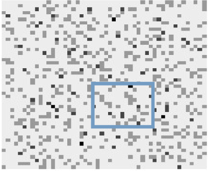
Figure 3: Patterns of disease spread: the darker shades indicate the regional pattern combining various Ising realisations. The rectangular frame indicates the uncertain region.
References:
[1] S. Zimeras, Y. Matsinos: “Bayesian Spatial Uncertainty Analysis, Energy and environment; Recent researches in environmental and geological sciences International conference”, 7th, Energy and environment, Recent researches in environmental and geological sciences; 377-385, 2012.
[2] S. Zimeras, Y. Matsinos: “Modelling Spatial Medical Data, Effective Methods for Modern Healthcare Service Quality and Evaluation”, IGI Global, 75-89, 2016.
[3] S. Zimeras: “Statistical models in medical image analysis”, Ph.D. Thesis, Leeds University, Department of Statistics, 1997.
[4] Katz, R. W. “Techniques for estimating uncertainty in climate change scenarios and impact studies”. Climate Research 20:167-185, 2002.
Please contact:
Stelios Zimeras, University of the Aegean, Greece
