


by Wouter M. Koolen (CWI & University of Twente), Shubhada Agrawal (IISc Bangalore) and Martin Larsson (CMU)
Could our data be sub-Gaussian noise? We explore rejecting that null hypothesis with the help of e-variables. We map the landscape of optimal e-variables against two-point alternatives.
In hypothesis testing, our goal is to reject a null hypothesis by finding evidence that contradicts it. In the framework of e-values, this evidence is measured by an e-variable – a non-negative random variable whose expectation under the null is at most one. To maximise our testing power, we seek the e-variable with the largest expected logarithmic growth under a chosen alternative distribution.
While the optimal e-variable against a simple point-null is just the likelihood ratio, composite null hypotheses are far more challenging. For convex sets of distributions, we understand the growth-optimal e-variables for Bernoulli trials, for distributions defined by finitely many moment constraints, and even the one-sided sub-phi class [1,2]. However, the case of sub-Gaussian distributions has remained a glaring omission.
Sub-Gaussianity is the workhorse of modern noise modelling. It defines a non-parametric, convex set of distributions – including the standard Gaussian and the discrete Rademacher distribution – characterised by a continuous family of moment constraints. This raises a fundamental question: How do we refute sub-Gaussianity using e-values?
One might expect to straightforwardly extend the solution for finitely many moment constraints. But one cannot. The reason lies in a mathematical “Easter egg” found in the definition of sub-Gaussianity itself. Indeed, any sub-Gaussian distribution has mean zero and variance bounded by one. Hence the outcome squared is an e-variable. Yet crucially, that square cannot be expressed as a mixture of the exponentials that define sub-Gaussianity. It emerges only through limits.
We recently characterised admissible sub-Gaussianity e-variables, as shown in the Figure. These variables are composed of a signed bet against the mean and positive bets against the sub-Gaussian constraints, reorganised to introduce a removable singularity (specifically, the limit as the constraint parameter approaches zero now results in the square).
Here we take this characterisation for a spin by numerically exploring the log-optimal e-variables for arbitrary two-point alternatives. Two-point distributions have three parameters (two points and one weight), and while we did all computations in 3d we can only present a 2d slice here. In the Figure we map the structure of these problems across the plane. Each coordinate represents a two-point alternative distribution, with the left and right support points on the axes and a fixed weight of 0.745 on the left point (a value chosen to reveal the most intricate structure). At each such alternative we computed the KKT saddle point, obtaining the primal e-variable and its dual, the RIPr (the reverse information projection, i.e. the sub-Gaussian distribution closest in KL-divergence to the alternative). Even though we are optimising over functions and measures, the major surprise here is that both primal and dual solutions have tractable short descriptions. The RIPr is supported on exactly three points: the two points of the alternative and a third optimised point where the optimal e-variable vanishes. The optimal e-variable puts weight only on the one or two active sub-Gaussianity constraints for the RIPr.
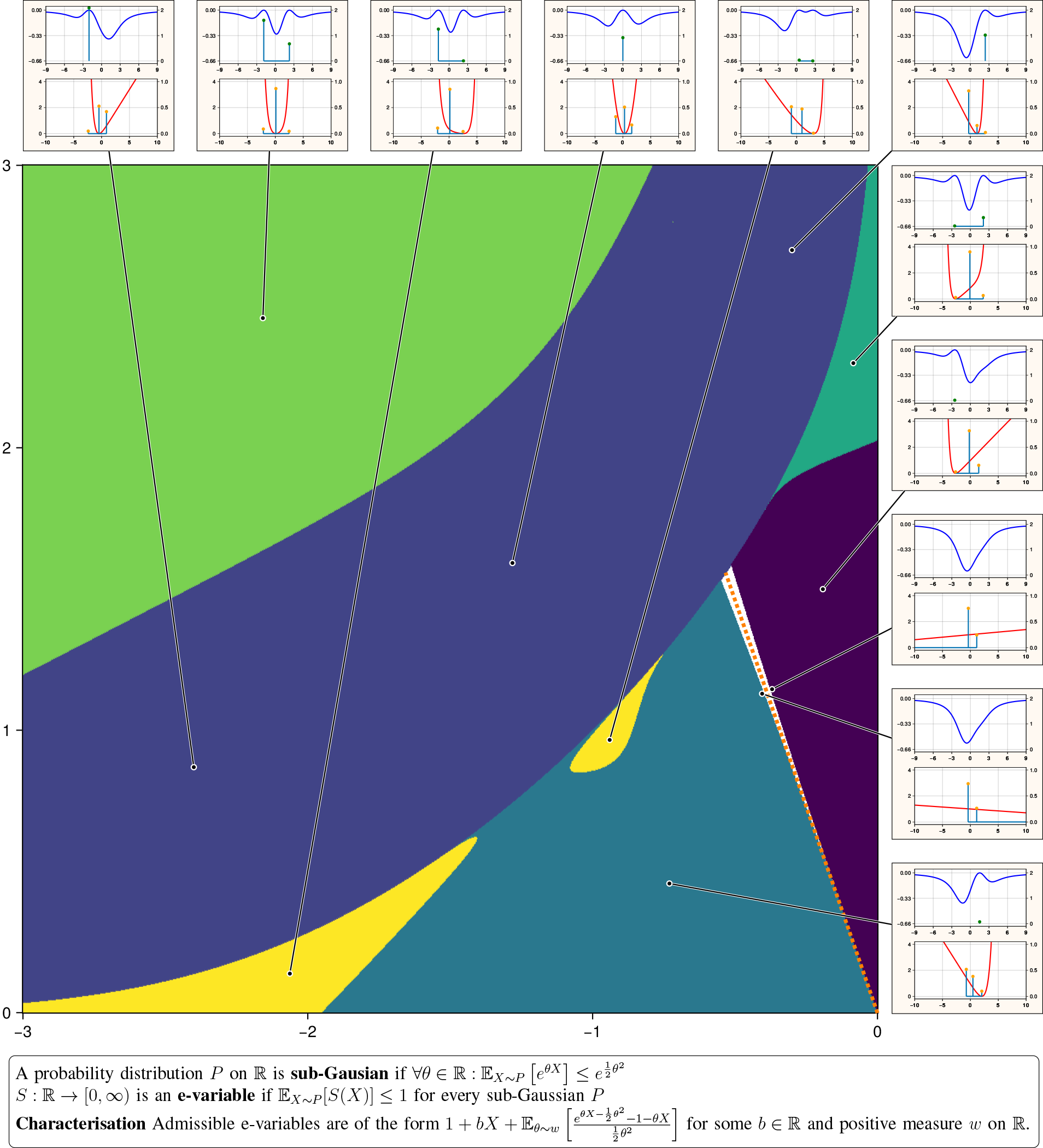
The Figure reveals the underlying geometry of the optimal e-variable, which bets against two constraints (yellow, green and teal), or against one (blue, turquoise and purple). Within each, the colours flag whether the third support point is located before, between or beyond the two support points of the alternative. For a selection of 11 alternative distributions, the log-optimal e-variable is graphed in red, together with the RIPr. In blue we graph the sub-Gaussianity constraints, together with the one- or two-point positive measure, which is supported precisely on the one or two points where the constraints are tight. In the white area our method runs into numerical trouble, as the third support point walks off to infinity and the optimal e-variable becomes the flat 1. The fourth selected alternative in the top row puts all mass on the sub-Gaussianity constraint at parameter value zero, where the optimal e-variable is indeed a parabola (betting against the outcome and the outcome squared). Due to our parametrisation this smoothly fits in the general pattern.
The upshot?
Beyond providing a rigorous sanity check for our characterisation, this work yields a parametric family of optimal e-variables defined by at most five parameters. This makes it possible to employ adaptive sequential learning methods when data arrives from any unknown two-point alternative. Our results pave the way for a full understanding of the landscape beyond two-point alternatives, and for practical efficient anytime-valid refutation of sub-Gaussianity.
Each point in the plane represents a two-point alternative distribution, defined by its left (x-axis) and right (y-axis) support points, with a fixed weight of 0.745 on the former. The distributions on the dotted orange line segment are sub-Gaussian, the rest is not. The colours categorise the structural regimes of the log-optimal e-variable and its dual, the RIPr. In the yellow, green, and teal regions, the e-variable bets against two constraints; in the blue, turquoise, and purple regions, it bets against only one. The insets show (bottom graphs) the e-variable in red together with the RIPr, which is supported on the two points of the alternative and a third special point where the e-variable vanishes. The insets further show (top graphs) the sub-Gaussianity constraints of the RIPr in blue, together with the mixture of bets employed by the optimal e-variable against the tight constraints, of which there can be either one or two (in some cases these fall outside the range of the x-axis). In the white area, the third support point escapes to infinity, while its mass tends to zero, causing the e-variable to flatten to 1 at the sub-Gaussian submodel (dotted orange).
Martin Larsson acknowledges support from NSF grant DMS-2510965.
References:
[1] P. Grünwald, R. de Heide, and W. Koolen, “Safe testing,” Journal of the Royal Statistical Society Series B:
Statistical Methodology, vol. 86, no. 5, pp. 1091–1128, Nov. 2024.
[2] M. Larsson, A. Ramdas, and J. Ruf, “Testing hypotheses generated by constraints,” Mathematics of Operations Research, vol. 0, no. 0, 2026.
Please contact:
Wouter Koolen
CWI and University of Twente, The Netherlands

