


by Ruodu Wang (University of Waterloo)
A model-free method lets regulators and financial institutions continuously monitor tail-risk forecasts using e-values that remain valid whenever checked.
After every market shock, the same question arises for financial institutions and regulators: were market-risk forecasts adequately computed and reported? Under the Basel regulatory framework [1], banks report daily risk measures that determine how much capital they must hold. Regulators, as well as banks themselves, then check whether these forecasts are consistent with data; this task is referred to as backtesting.
Backtesting risk forecasts is almost as old as measuring financial risk itself. For a long time, the main target in finance was Value-at-Risk (VaR). In simple terms, VaR is a high-level, usually 99%, quantile of the future loss distribution over a fixed horizon. It has a simple model-free backtesting culture: count the days on which losses exceed the forecast. This requires a fixed testing period; in statistical jargon, it is not an online method and does not naturally handle data arriving sequentially, typically every trading day. The first challenge is how to backtest risk forecasts online.
The task became much harder when Expected Shortfall (ES), defined as the expected loss given that the loss has reached a high level, replaced VaR as the standard risk measure for market risk in Basel’s 2019 regulatory framework. ES looks into the tail and captures the severity of large losses, which is why it is favoured by regulators and risk management scholars. It has also become popular in many areas involving risk assessment, including portfolio selection, robust optimisation, and machine learning. But this extra tail sensitivity comes at a statistical cost: ES does not admit a simple model-free backtesting procedure like VaR, even with a fixed data collection horizon. Thus, the second challenge is how to backtest ES in a model-free manner.
Evidence that can be checked at any time
With Qiuqi Wang and Johanna Ziegel, we developed the methodology of e-backtesting [2], a procedure that uses e-values and e-processes to monitor risk forecasts sequentially. An e-value can be read as the payoff of a fair bet against the hypothesis that the forecasts are adequate. If that hypothesis is true, the expected payoff is at most one. Multiplying daily e-values gives an evidence process whose guarantee is anytime-valid: a regulator or risk manager may look today, tomorrow or after a crisis week without invalidating the test. If the e-process crosses a threshold, the probability of such a false alarm under adequate forecasting is controlled by that threshold, no matter when the crossing occurs. This differs from a conventional p-value workflow, where tests are calibrated for one planned analysis and repeated peeking can distort error guarantees.
Addressing both challenges at once
The paper [2] introduces backtest e-statistics for risk-measure forecasts and characterises essentially unique optimal choices for VaR and for the ES-VaR pair. Each day’s loss and forecasts are converted into an e-value. Conservative forecasts, which are acceptable in prudential regulation, keep the process low; forecasts that repeatedly fall short of realised tail risk push it upward.
This methodology leaves flexibility in how the e-process is constructed. To make it powerful in practice, we propose data-driven rules that approximate a growth-rate-optimal principle for e-processes. The recommended default, GREM, combines two adaptive strategies and performs competitively while avoiding assumptions on the forecasting mechanism and the loss distributions.
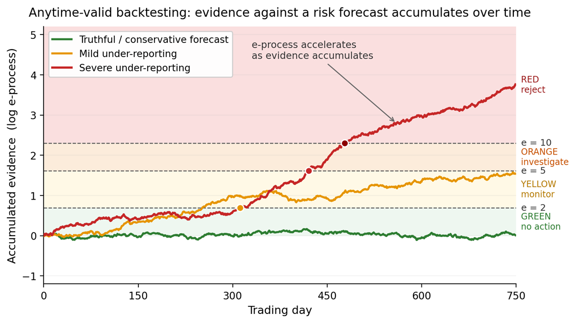
Because evidence accumulates gradually, the method naturally supports a multi-zone alarm system. A regulator could treat moderate thresholds as early warnings, higher thresholds as substantial evidence, and still higher thresholds as decisive evidence. The interface could be one curve per institution: green for no action, yellow for monitoring, orange for investigation and red for rejection (Figure 1).
What happens on market data
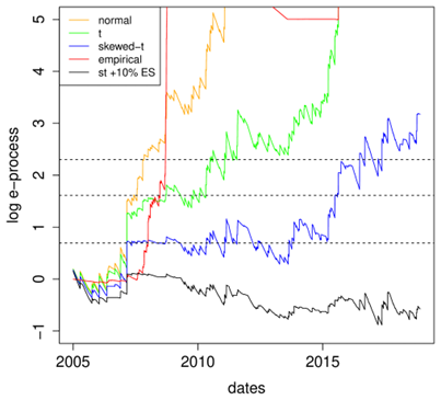
As a simple example, we applied the method to daily NASDAQ Composite returns from January 2005 to December 2021. Several standard forecast methods produced 97.5% ES forecasts. Empirical and AR-GARCH forecasts with Gaussian innovations were rejected decisively within months of the 2007-2008 financial crisis. Forecasts based on Student-t or skewed-t innovations survived longer but eventually accumulated evidence against them. A deliberately conservative forecast, set 10% above the skewed-t estimate, was not rejected (Figure 2).
This is the behaviour a regulatory backtest should encourage. The method is not trying to punish cautious capital estimates, nor does it presume bad intent. It seeks persistent evidence that forecasts are inadequate, whether because of model misspecification, structural change, statistical difficulty or under-reporting. Even a skewed-t AR-GARCH model, often regarded as a strong model for financial log-returns, still underestimated the market risk in this period.
Beyond banking
Although motivated by financial regulation, the same idea applies more broadly, as shown by the theory developed in the paper. Whenever a forecast target, such as the mean, the variance, or another risk measure, admits a suitable backtest e-statistic, an e-process can turn repeated forecast evaluation into an anytime-valid monitoring tool. E-backtesting marks a shift from fixed-deadline tests to cumulative evidence that respects how decisions are actually made.
References:
[1] Basel Committee on Banking Supervision: Minimum Capital Requirements for Market Risk. BIS, 2019. https://www.bis.org/bcbs/publ/d457.pdf
[2] Q. Wang, R. Wang and J. Ziegel, “E-backtesting”,
Management Science, 72(6):4952-4973, 2026. https://doi.org/10.1287/mnsc.2023.01659
Please contact:
Ruodu Wang
Department of Statistics and Actuarial Science
University of Waterloo, Canada

