


Mathematicians are particularly attracted by the deep connection between this problem and several esoteric fields of functional analysis and variational calculus. Digital images are commonly presented as matrices of scalars for grey-scale images or vectors for colour images. These matrices are seen as the values of a distribution (generalized function) u0(x) defined on an open and bounded 2D domain Ω. This allows a functional analytic setting for image-processing problems and in particular, for the design of digital processing algorithms through partial differential equation models.
In their book (T. Chan and J. Shen, 'Image Processing and Analysis', SIAM, 2005) Chan and Shen give several examples of mathematical models of noise and describe images as distributions. In this framework, the denoising process can be modelled by variational problems.
One popular model for image denoising is Rudin, Osher and Fatemi's model, where we seek a distribution u(x) in the space of the Bounded Variation (BV) distributions, which is the solution to the following nonlinear minimization problem (1):
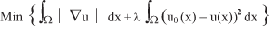
Here, W is the unit square for the sake of simplicity and u0(x) is the image affected by Gaussian white noise.
It is standard to seek a solution to (1) by solving a related nonlinear parabolic equation using a pseudo-time-stepping algorithm in order to approximate the steady-state configuration u(x).
Another possible model we are currently investigating can be described by the use of fractional Sobolev spaces Hα, 0 < α <1. An exhaustive presentation of these spaces can be found in the first book of Lions and Magenes (J. L. Lions and E. Magenes, 'Problèmes aux limites non homogènes et applications', Dunod, 1968). In this denoising model we seek a distribution u(x) ∈ Hα which is the solution of a quadratic minimization problem (2).
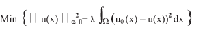
Problem (2) is approximated by a finite-element method that produces the linear system of equations (Sα + λI) u = λu0, where we need to compute the a power of a special matrix S. Owing to the large size of the problem, the numerical solution to this problem is computed by an iterative solver that uses a Lanczos method applied to a generalized eigenvalue problem in order to approximate Sα.
 original image; b) noisy image; c) denoised image using method (1); d) denoised image using method (2).")
These methods are illustrated in Figure 1. In a) we give an example of an image with a resolution of 512x512 pixels; in b) we show the same image with the addition of random white noise. The size of the matrices and vectors arising from both methods is 5122=262,144. Both methods were considered with the same value of the regularising parameter λ=1/50. In c), we show the result computed using method (1) via a Matlab implementation provided by Pascal Getreuer (2007). In d) we show the result computed using method (2) for α=0.5.
Please contact:
Mario Arioli
STFC, UK
E-mail: m.arioli![]() rl.ac.uk
rl.ac.uk
Daniel Loghin
University of Birmingham
E-mail: d.loghin![]() bham.ac.uk
bham.ac.uk
